China mainland population density

Required libraries

We need several R packages for this study.

library(maptools)
library(rgdal)
library(raster)
library(ggplot2)
library(ggthemes)

Get and clean population and grid data

The data is available for free to download on SEDAC website https://sedac.ciesin.columbia.edu/data/set/gpw-v3-population-density

Please note that the Trustees of Columbia University in the City of New York and the Centro Internacional de Agricultura Tropical (CIAT) hold the copyright of this dataset. Users are prohibited from any commercial, non-free resale, or redistribution without explicit written permission from CIESIN or CIAT. Users should acknowledge CIESIN and CIAT as the source used in the creation of any reports, publications, new data sets, derived products, or services resulting from the use of this data set.

There are 3 formats available: .bil, .ascii or .grid (https://en.wikipedia.org/wiki/Esri_grid) We will use directly the ASCII version which can be read with readAsciiGrid() from the maptool package.

We select data for China only and download 1 datasets : Population density grid; We use a cached version stored on datapleth.io cloud and load the file raster.

# chnds00g  population densities in 2000, unadjusted, persons per square km
densGriCountFile <- "https://data.datapleth.io/ext/gridded-Population-of-China/chndens-ascii/chnds00g.asc"
download.file(
  url = densGriCountFile, 
  destfile = "./data/chnds00g.asc", 
  method = "wget", quiet = TRUE,
  mode = "w", cacheOK = TRUE
)
dens <- raster::raster("./data/chnds00g.asc")
raster::fromDisk(dens)

## [1] TRUE

Visualise gridded data

plot(dens, main="China population density grid")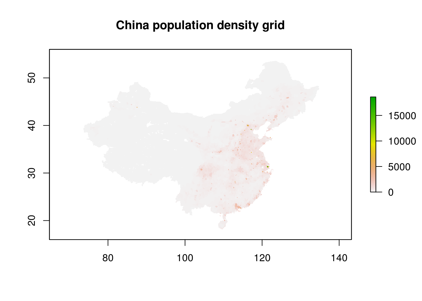

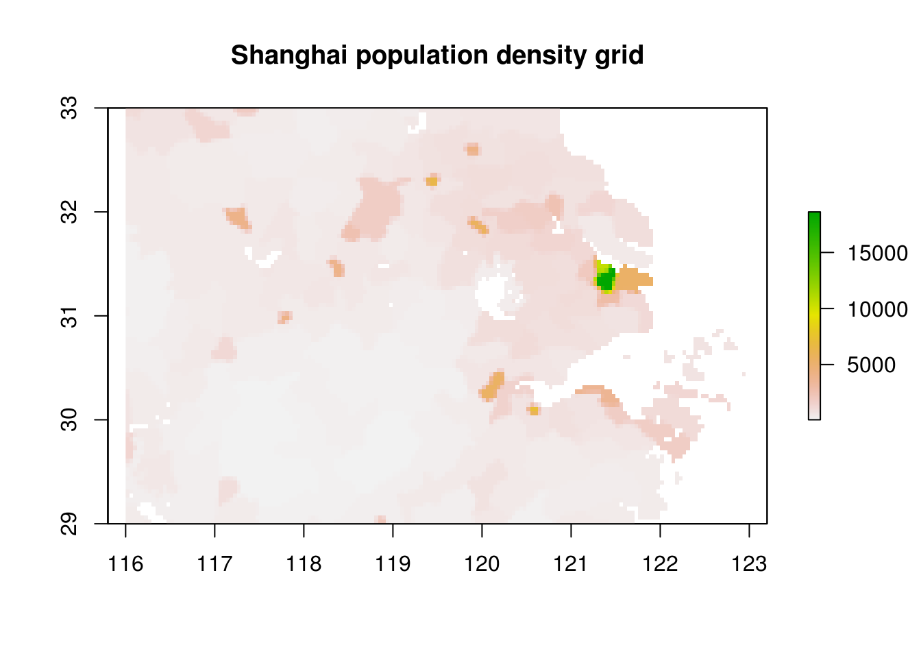
# Around Shanghai
plot(
  crop(
    dens,
    c(116, 123, 29, 33)
  ),
  main="Shanghai population density grid"
)

Toward a map of China density

We first load China map with regions (see earlier post)

ChinaPolygonsLevel1 <- rgdal::readOGR("./data/CHN_adm1.shp")

## OGR data source with driver: ESRI Shapefile 
## Source: "/home/travis/build/longwei66/datapleth/content/blog/data/CHN_adm1.shp", layer: "CHN_adm1"
## with 31 features
## It has 9 fields
## Integer64 fields read as strings:  ID_0 ID_1

## Fix English names, simplify
ChinaPolygonsLevel1@data$NAME_1 <- as.character(ChinaPolygonsLevel1@data$NAME_1)
ChinaPolygonsLevel1@data[grep("Xinjiang Uygur", ChinaPolygonsLevel1@data$NAME_1),]$NAME_1 <- "Xinjiang"
ChinaPolygonsLevel1@data[grep("Nei Mongol", ChinaPolygonsLevel1@data$NAME_1),]$NAME_1 <- "Nei Menggu"
ChinaPolygonsLevel1@data[grep("Ningxia Hui", ChinaPolygonsLevel1@data$NAME_1),]$NAME_1 <- "Ningxia"
ChinaPolygonsLevel1@data$NAME_1 <- as.factor(ChinaPolygonsLevel1@data$NAME_1)

# Use level1 as index & Province name as id
ChinaLevel1Data <- ChinaPolygonsLevel1@data
ChinaLevel1Data$id <- ChinaLevel1Data$NAME_1

# Fortify the data (polygon map as dataframe) using english names
ChinaLevel1dF <- ggplot2::fortify(ChinaPolygonsLevel1, region = "NAME_1")

## Merge polygons and associated data in one data frame by id (name of the province in chinese)
ChinaLevel1 <- merge(ChinaLevel1dF, ChinaLevel1Data, by = "id")
rm(ChinaPolygonsLevel1, ChinaLevel1dF, ChinaLevel1Data)

Then we convert the density raster data to data.frame in order to use ggplot in the next steps.

## convert the raster to points (to plot with ggplot)
raster_points_dens <- raster::rasterToPoints(dens)
raster_points_dens <- data.frame(raster_points_dens)
colnames(raster_points_dens) <-c('x','y','density')

We make a first plot.

md <- ggplot(data=raster_points_dens, aes(y=y, x=x)) 
md <- md + geom_raster(aes(fill=density))
md + scale_fill_gradient(low="white", high="blue")

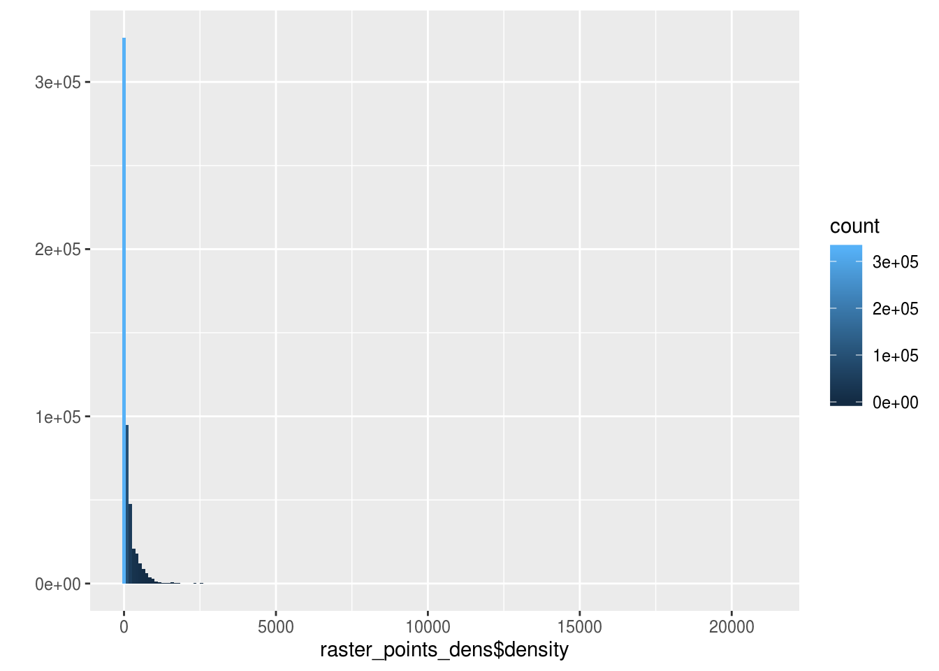
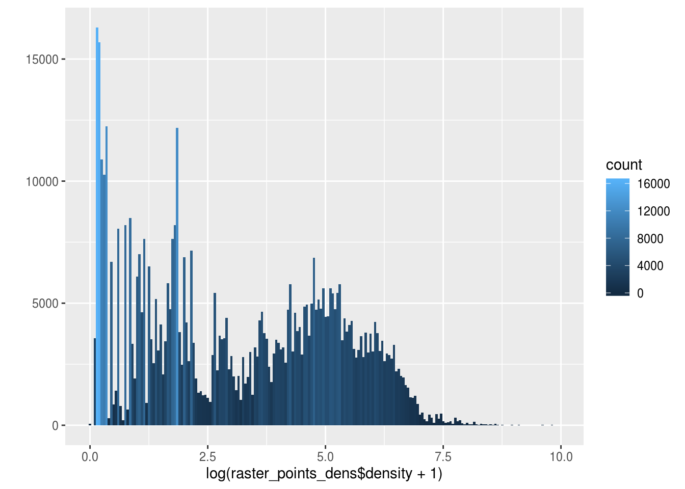
The problem of this visualisation is the large extend of distribution of densities. China is definitely a wide country which is dense and empty at the same time ! So we switch to a log scale to get a better vizualisation.

qplot(
  x = raster_points_dens$density,
  fill=..count.., 
  geom="histogram",
  bins = 200
)

qplot(
  x = log(raster_points_dens$density+1),
  fill=..count.., 
  geom="histogram",
  bins = 200
) 

Map of China density grid

As described above, we use a log(x+1) scale for the color scale (using trans="log1p") in the geom_raster.

g <- ggplot() + theme_tufte() +
  ## Projected shadows
  geom_polygon(
    data = ChinaLevel1,
    aes(x = long + 0.7, y = lat - 0.5, group = group),
    color = "grey50", size = 0.1, fill = "grey50"
  ) +
  ## Add Raster
  geom_raster(
    data=raster_points_dens,
    aes(y=y, x=x, fill=density)
  ) +
  scale_fill_distiller(
    palette = "Spectral",
    trans="log1p",
    breaks = c(0, 3, 10, 50, 200, 1000, 5000, 20000)
  ) +
  ## Province boundaries
  geom_polygon(
    data = ChinaLevel1,
    aes( x = long, y = lat, group = group, fill = NULL),
    alpha = 0.01, color = "black", size = 0.2
  ) +
  ## Styling
  labs(title = "China mainland - population density & provinces") +
  theme( axis.text=element_blank(), axis.ticks=element_blank(),
         axis.title=element_blank())
print(g)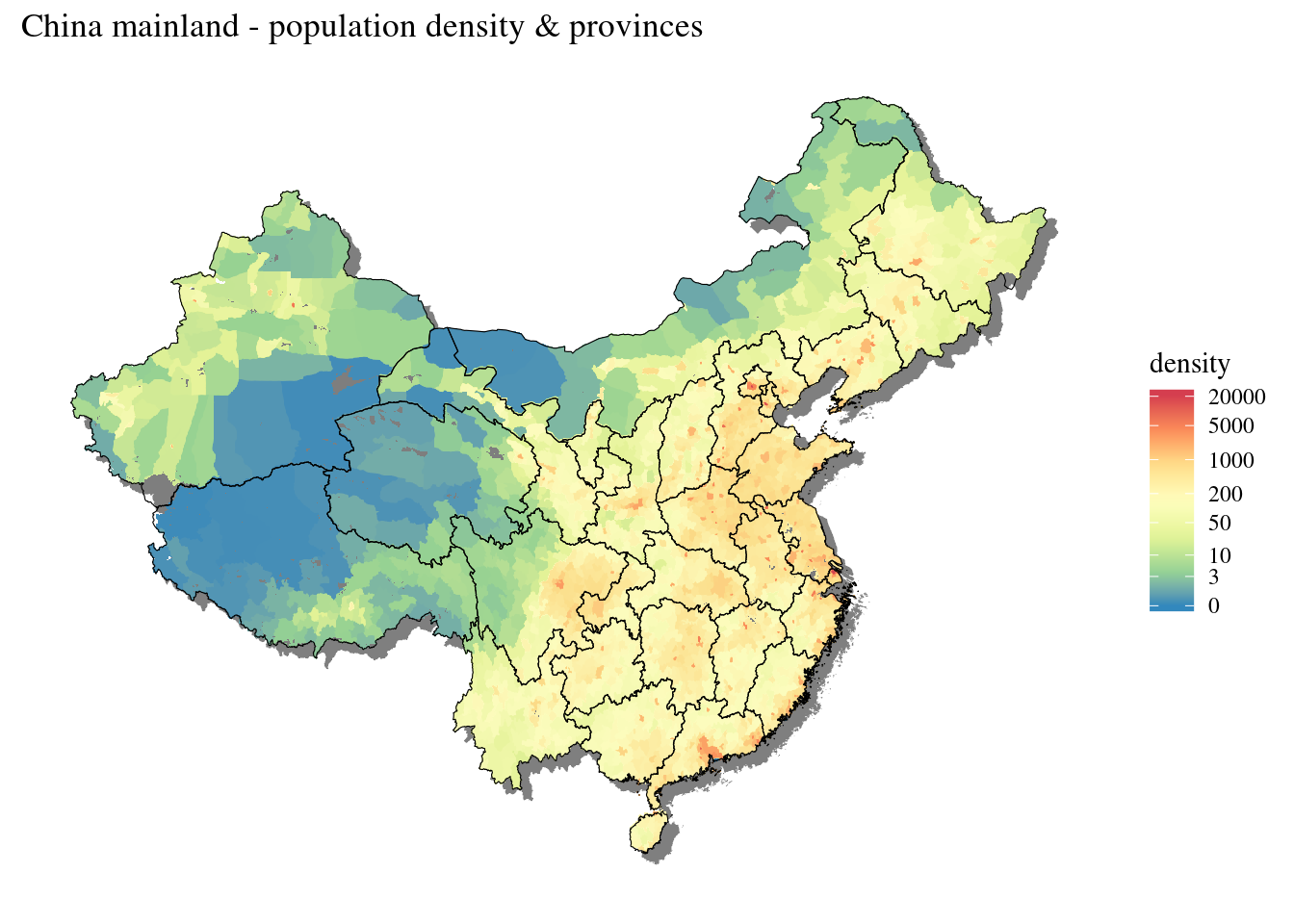

References

Source
Center for International Earth Science Information Network - CIESIN - Columbia University, United Nations Food and Agriculture Programme - FAO, and Centro Internacional de Agricultura Tropical - CIAT. 2005. Gridded Population of the World, Version 3 (GPWv3): Population Count Grid. Palisades, NY: NASA Socioeconomic Data and Applications Center (SEDAC). https://doi.org/10.7927/H4639MPP. Accessed 2019-12-12.
Other example of use of raster package
https://pakillo.github.io/R-GIS-tutorial/#raster http://zevross.com/blog/2015/03/30/map-and-analyze-raster-data-in-r/ https://jeffreybreen.wordpress.com/tag/raster/