By Datapleth.io | October 19, 2015
In this article we are going to plot a map of China urbanization rate per provinces together with Chinese cities with at least 2 millions population.
In a nutshell, we’ll get first rural and urban population data from official China statistic bureau, then clean the data, we’ll repeat the same two steps for Chinese largest cities. Secondly, we’ll prepare a map of China with provinces. Then we will add the main Chinese cities and their population and a choropleth of urbanization rate, add main cities
library(reshape2)
library(ggplot2)
library(maptools)
library(maps)
library(knitr)
library(kableExtra)
library(dplyr)
Rural and urban population of China
The best source we found is the official China statistic bureau. You can follow the following link to download the data : http://data.stats.gov.cn/english/
We will need three files, Rural, Urban and Total resident per provinces.
Population data for 2000 and 2001 are estimated on the basis of population census, the rest of the data are estimated on the basis of the annual national sample surveys on population changes. Population data by region are permanent resident population since 2005.
## data.stats.gov.cn files tend to be formatted with similar patterns
loadPolupationData <- function(dataFile,mapVariable = "population"){
        dF <- read.csv(dataFile ,header = TRUE, stringsAsFactors = FALSE, skip = 3)
        ## Remove NA values
        dF <- dF[complete.cases(dF),]
        ## Melt as long format
        dF <- melt(dF, id.vars = "Region")
        ## get the proper year format
        dF$variable <- as.numeric(gsub("^X", "", dF$variable))
        ## get the proper province names
        dF$Region <- gsub("^Inner Mongolia$", "Nei Menggu", dF$Region)
        dF$Region <- gsub("^Tibet$", "Xizang", dF$Region)
        ## Get the population in million of people
        dF$value <- (dF$value * 10000)/1000000
        names(dF) <- c("Region", "Year", mapVariable)
        dF }
provincePopulationT <- loadPolupationData(
dataFile = "https://data.datapleth.io/ext/province-population/China-Total-Resident-per-province.csv",
mapVariable = "Total.Population"
)
provincePopulationU <- loadPolupationData(
dataFile = "https://data.datapleth.io/ext/province-population/China-Urban-Resident-per-province.csv",
mapVariable = "Urban.Population"
)
provincePopulationR <- loadPolupationData(
dataFile = "https://data.datapleth.io/ext/province-population/China-Rural-Resident-per-province.csv",
mapVariable = "Rural.Population"
)
## merge in one data frame
provincePopulation <- merge(provincePopulationT, provincePopulationU)
provincePopulation <- merge(provincePopulation, provincePopulationR)
rm(provincePopulationR, provincePopulationT, provincePopulationU)
## Add index
provincePopulation$Urbanisation.rate <- provincePopulation$Urban.Population / provincePopulation$Total.Population
## Melt as long format
provincePopulation <- melt(provincePopulation, id.vars = c("Region", "Year"))We use a generic function to load and clean the data and we plot an overview bellow in a quick bar plot :
## select urbanisation rate as variable
dF <- provincePopulation[provincePopulation$variable =="Urbanisation.rate",]
## fix the order using 2014 reference by urbanisation rate decreasing
ordered.label <- dF[order(dF$variable, dF$value) , ]
ordered.label <- ordered.label[ordered.label$Year == "2014",]$Region

g <- ggplot(dF, aes(x=Region, y=value)) +
        geom_bar(stat = "identity", fill="chartreuse4") +
        coord_flip() + facet_grid(facets = . ~ Year) +
        scale_x_discrete( limits=ordered.label ) +
        theme(axis.text.x = element_text(angle = 90))
print(g)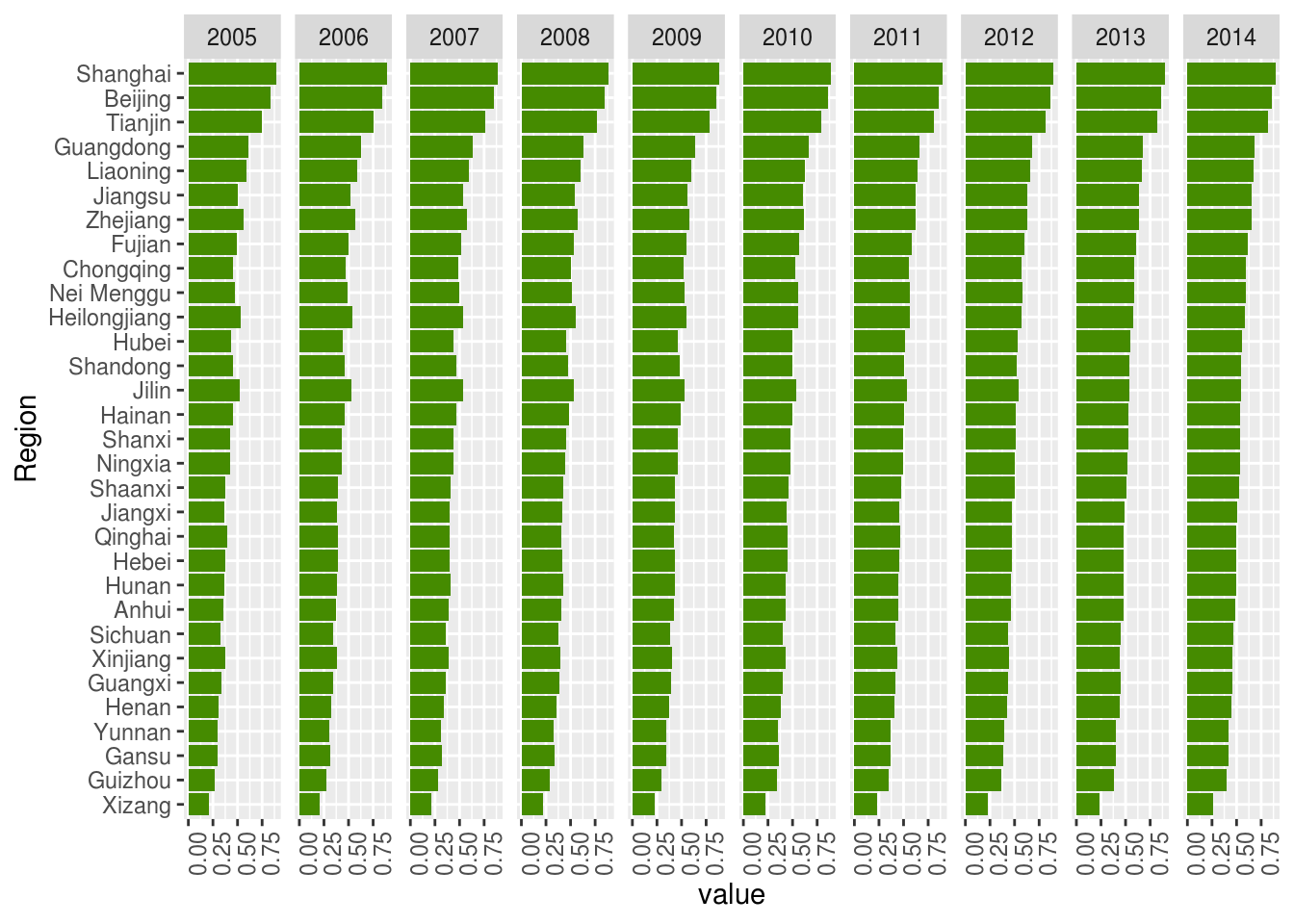
Map of China with provinces, municipalities and autonomous regions
We need now to load the polygon shape data frame for china level one subdivisions, merge it with urbanization rate data.
ChinaPolygonsLevel1 <- maptools::readShapeSpatial(fn = "./data/CHN_adm1.shp")

## Fix English names, simplify
ChinaPolygonsLevel1@data$NAME_1 <- as.character(ChinaPolygonsLevel1@data$NAME_1)
ChinaPolygonsLevel1@data[grep("Xinjiang Uygur", ChinaPolygonsLevel1@data$NAME_1),]$NAME_1 <- "Xinjiang"
ChinaPolygonsLevel1@data[grep("Nei Mongol", ChinaPolygonsLevel1@data$NAME_1),]$NAME_1 <- "Nei Menggu"
ChinaPolygonsLevel1@data[grep("Ningxia Hui", ChinaPolygonsLevel1@data$NAME_1),]$NAME_1 <- "Ningxia"
ChinaPolygonsLevel1@data$NAME_1 <- as.factor(ChinaPolygonsLevel1@data$NAME_1)

# Use level1 as index & Province name as id
ChinaLevel1Data <- ChinaPolygonsLevel1@data
ChinaLevel1Data$id <- ChinaLevel1Data$NAME_1

# Fortify the data (polygon map as dataframe) using english names
ChinaLevel1dF <- fortify(ChinaPolygonsLevel1, region = "NAME_1")

## Merge polygons and associated data in one data frame by id (name of the province in chinese)
ChinaLevel1 <- merge(ChinaLevel1dF, ChinaLevel1Data, by = "id")
rm(ChinaPolygonsLevel1, ChinaLevel1dF, ChinaLevel1Data)

## Create the ggplot using standard approach
## group is necessary to draw in correct order, try without to understand the problem
g <- ggplot(ChinaLevel1, aes(x = long, y = lat, fill = ENGTYPE_1, group = group))
## projected shadow
g <- g+ geom_polygon(aes(x = long + 0.7, y = lat - 0.5), color = "grey50", size = 0.2, fill = "grey50")
## Province boundaries
g <- g + geom_polygon(color = "white", size = 0.2)
## to keep correct ratio in the projection
g <- g + coord_map()
g <- g + labs(title = "China - level 1 subdivisions")
print(g)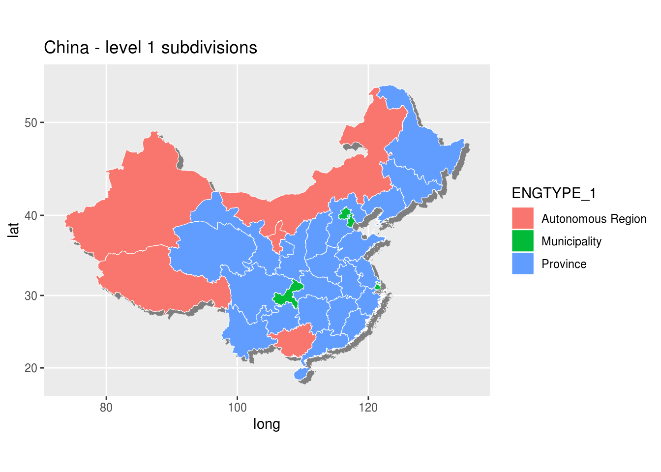
Main Chinese Cities data
We want to add on the map the main Chinese cities with their population. There
are multiple sources for such data but most of them requires intensive data
processing. This will be the topic of another article. For this post, let’s use
available data in R and the world.cities data set of the packages maps.
data("world.cities")
## Get cities of China
mainCitiesOfChina <- world.cities[world.cities$country.etc == "China",]
## convert population in millions
mainCitiesOfChina$pop <- mainCitiesOfChina$pop / 1000000
Let’s have a look on the data.
# we use kable to generate an html table with nice formatting
knitr::kable(head(mainCitiesOfChina[mainCitiesOfChina$pop > 2,],4)) %>%
  kable_styling(
    bootstrap_options = c(
      "striped"
      , "hover"
      , "condensed"
      , "responsive"
      )
) %>% scroll_box(width = "100%")| name | country.etc | pop | lat | long | capital | |
|---|---|---|---|---|---|---|
| 3826 | Beijing | China | 7.602069 | 39.93 | 116.40 | 1 |
| 7108 | Changchun | China | 2.602574 | 43.87 | 125.35 | 3 |
| 7118 | Changsha | China | 2.131620 | 28.20 | 112.97 | 3 |
| 7271 | Chengdu | China | 3.961709 | 30.67 | 104.07 | 3 |
Plot China map
We will proceed in two steps, we will make first a choropleth by province of urbanization rate and then we will add cities.
Provinces, urbanisation rate choropleth
We should map the urbanization rate from the provincePopulation dataframe with
province of the maps defined by ChinaLevel1. Let’s first check that all
provinces are covered and names are matching.
a <- unique(provincePopulation[provincePopulation$variable == "Urbanisation.rate",]$Region)
b <- unique(ChinaLevel1$id)
all(a %in% b)
## [1] TRUEThis looks good, we can proceed and plot the map.
## get large version of the urbanisation dataset
provincesUrbanisation <- dcast(provincePopulation, Year + Region ~ variable, value.var = "value")
## Merge polygons and associated urbanisation data in one data frame by id (name of the province in chinese) and Region - Only for year 2014
urbanisationChoropleth <- merge(ChinaLevel1, provincesUrbanisation[provincesUrbanisation$Year == "2014",], by.x = "id", by.y = "Region")
rm(ChinaLevel1)

## Create the ggplot using standard approach
## group is necessary to draw in correct order, try without to understand the problem
g <- ggplot(
        urbanisationChoropleth,
        aes(x = long, y = lat, fill = Urbanisation.rate, group = group)
        )
g <- g + scale_fill_continuous(na.value = "grey80", low = "#ffdddd", high = "#ff3311", name = "Urbanization %")
## projected shadow
g <- g + geom_polygon(aes(x = long + 0.7, y = lat - 0.5), color = "grey50", size = 0.2, fill = "grey50")
## Province boundaries
g <- g + geom_polygon(color = "white", size = 0.2)
## to keep correct ratio in the projection
g <- g + coord_map()
g <- g + labs(title = "China - Urbanisation rate")
print(g)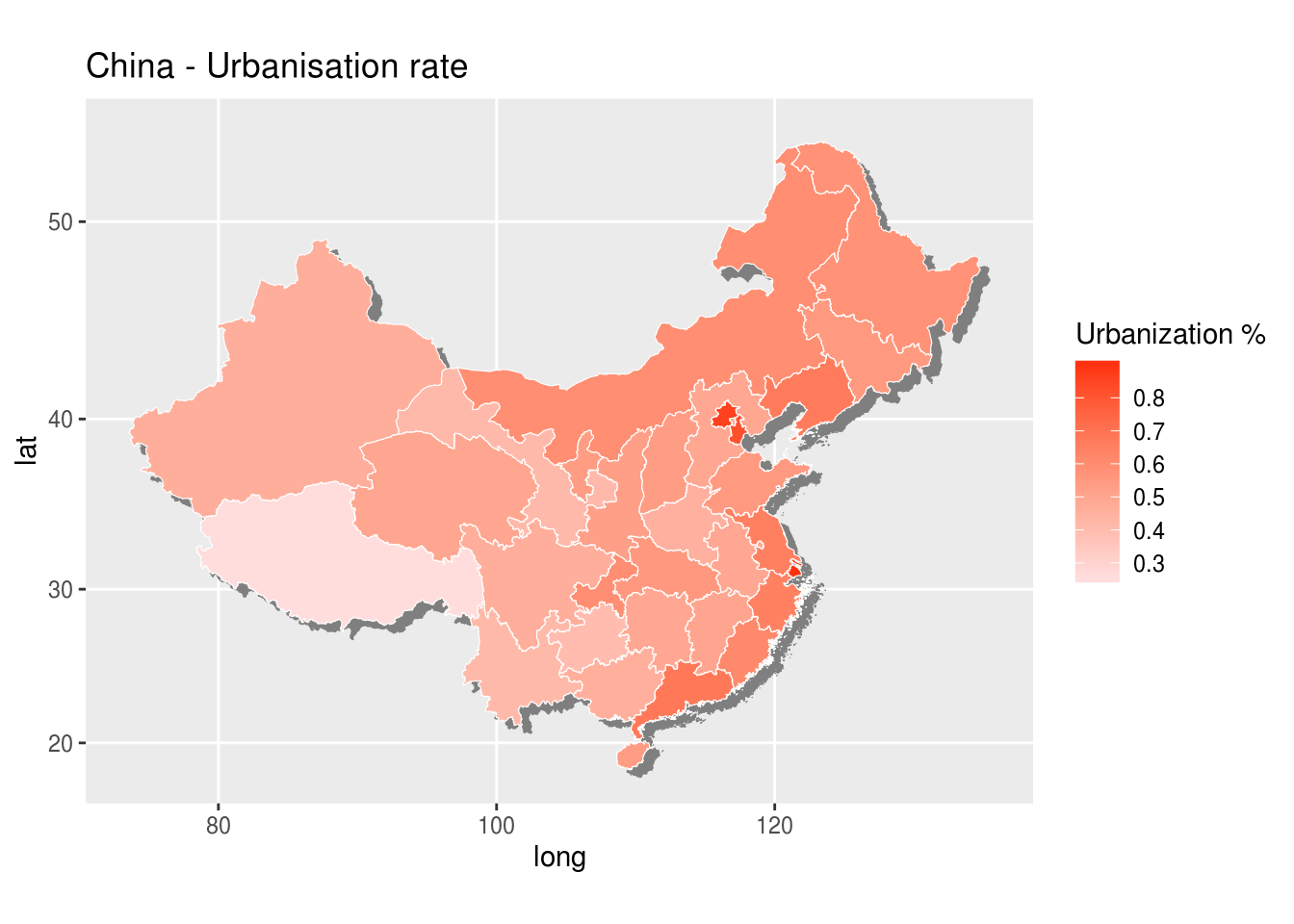
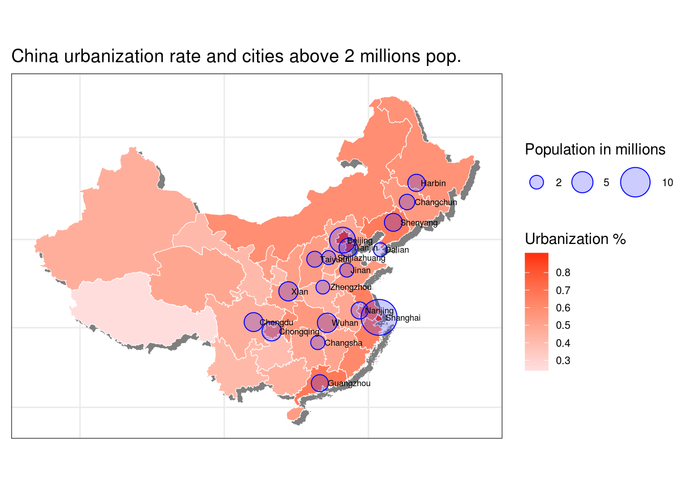
Adding Largest cities
Then we just need to add another layer with bubbles for each cities larger than 2 millions inhabitants.
## Theme configuration, as simple a possible
r <- g + theme_bw() + theme(axis.text = element_blank(),
              axis.title = element_blank(),
              axis.ticks = element_blank(),
              legend.text = element_text(size = rel(0.7))
              )
## Bubles for cities, we superpose two type of geom_point, circles an disks with alpha
r <- r + geom_point(
        data = mainCitiesOfChina[mainCitiesOfChina$pop > 2,],
        aes(x = long, y = lat, size = pop, fill = NULL, group = NULL ),
        colour = "blue", alpha = 1, pch = 1
        )
r <- r + geom_point(
        data = mainCitiesOfChina[mainCitiesOfChina$pop > 2,],
        aes(x = long, y = lat, size = pop, fill = NULL, group = NULL ),
        colour = "blue", alpha = 0.2, pch = 16
        )
r <- r + scale_size_area(max_size = 12, breaks = c(2,5,10), name = "Population in millions")
## Add city names, hjust is a small adjustment for better readability
r <- r + geom_text(
        data = mainCitiesOfChina[mainCitiesOfChina$pop > 2,],
        aes(x = long, y = lat, label = name, size = 0.5, group = NULL, fill = NULL, hjust = -0.18),
        show.legend = FALSE
        )
r <- r + guides(colour = guide_legend(nrow = 2), size =  guide_legend(order = 1, nrow = 1))
r <- r + labs(title = "China urbanization rate and cities above 2 millions pop.")
print(r)
Code information
Source code
The source code of this post is available on github
Session information
sessionInfo()## R version 3.6.1 (2017-01-27)
## Platform: x86_64-pc-linux-gnu (64-bit)
## Running under: Ubuntu 16.04.6 LTS
##
## Matrix products: default
## BLAS: /home/travis/R-bin/lib/R/lib/libRblas.so
## LAPACK: /home/travis/R-bin/lib/R/lib/libRlapack.so
##
## locale:
## [1] LC_CTYPE=en_US.UTF-8 LC_NUMERIC=C
## [3] LC_TIME=en_US.UTF-8 LC_COLLATE=en_US.UTF-8
## [5] LC_MONETARY=en_US.UTF-8 LC_MESSAGES=en_US.UTF-8
## [7] LC_PAPER=en_US.UTF-8 LC_NAME=C
## [9] LC_ADDRESS=C LC_TELEPHONE=C
## [11] LC_MEASUREMENT=en_US.UTF-8 LC_IDENTIFICATION=C
##
## attached base packages:
## [1] stats graphics grDevices utils datasets methods base
##
## other attached packages:
## [1] dplyr_0.8.3 kableExtra_1.1.0 knitr_1.26 maps_3.3.0
## [5] maptools_0.9-9 sp_1.3-2 ggplot2_3.2.1 reshape2_1.4.3
##
## loaded via a namespace (and not attached):
## [1] tidyselect_0.2.5 xfun_0.11 purrr_0.3.3 lattice_0.20-38
## [5] colorspace_1.4-1 vctrs_0.2.0 htmltools_0.4.0 viridisLite_0.3.0
## [9] yaml_2.2.0 rlang_0.4.2 pillar_1.4.2 foreign_0.8-72
## [13] glue_1.3.1 withr_2.1.2 lifecycle_0.1.0 plyr_1.8.5
## [17] stringr_1.4.0 rgeos_0.5-2 munsell_0.5.0 blogdown_0.17.1
## [21] gtable_0.3.0 rvest_0.3.5 mapproj_1.2.6 codetools_0.2-16
## [25] evaluate_0.14 labeling_0.3 highr_0.8 Rcpp_1.0.3
## [29] readr_1.3.1 scales_1.1.0 backports_1.1.5 webshot_0.5.2
## [33] farver_2.0.1 hms_0.5.2 digest_0.6.23 stringi_1.4.3
## [37] bookdown_0.16 grid_3.6.1 tools_3.6.1 magrittr_1.5
## [41] lazyeval_0.2.2 tibble_2.1.3 crayon_1.3.4 pkgconfig_2.0.3
## [45] zeallot_0.1.0 xml2_1.2.2 assertthat_0.2.1 rmarkdown_1.18
## [49] httr_1.4.1 rstudioapi_0.10 R6_2.4.1 compiler_3.6.1