The new french election geography

Election results

We need first to download the official results from data.gouv.fr. The data provided from the french government is not directly usable and we will have to clean and reshape. Some alternatives exists on open data portals but we prefer get the source data directly.

# load election results data
results_uri <- "https://www.data.gouv.fr/en/datasets/r/35170deb-e5f3-4e79-889f-5b9a3f547742"
election_results <- data.table::fread(
  results_uri, encoding = "Latin-1", dec= ","
)

The election result file does not contain the insee code of the “communes” (an equivalent of counties in USA). This information will be necessary to merge the results with the detailled map of France. Thus, we have to build this code using department number and commune code. This is working well except for data outside France mainland.

## ZZ for other countries -> 99
election_results[ , insee := as.numeric(`Code du département`)]
election_results[ 
  `Code du département` == "ZZ",
  insee := 99
  ]
election_results[ 
  `Code du département` %in% c("ZX","ZS","ZM","ZD","ZC","ZB","ZA"),
  insee := 97
  ]
election_results[ 
  `Code du département` %in% c("ZW","ZP","ZN"),
  insee := 98
  ]
election_results[, insee := as.character(insee*1000 + `Code de la commune`)]
election_results[ nchar(insee) == 4, insee := paste0("0",insee)]

The format of the data we obtained is really awfull, headers are not covering all columns. We first select the interesting columns and rename. We’ll use first the results of the main lists. Communes data are store in columns 1 to 18, then each list results are stored in 7 columns.

extract_list <- function(data,list_id = 23){
  # compute list index and extract it
  idx <-  c(1:18, (19+(list_id -1)*7):(19+(list_id -1)*7+6),257)
  sub_data <- data[ , .SD, .SDcols=idx]
  names_clean <- c(
    "departement_id", #[1] "Code du département"   
    "deparement_name", #[2] "Libellé du département"
    "commune_id", #[3] "Code de la commune"    
    "commune_name", #[4] "Libellé de la commune" 
    "inscrits", #[5] "Inscrits"              
    "abstentions", #[6] "Abstentions"           
    "absentions_perc", #[7] "% Abs/Ins"             
    "votants", #[8] "Votants"               
    "votants_perc", #[9] "% Vot/Ins"             
    "blancs", #[10] "Blancs"                
    "blancs_perc", #[11] "% Blancs/Ins"          
    "blancs_perc_votants", #[12] "% Blancs/Vot"          
    "nuls", #[13] "Nuls"                  
    "nuls_perc", #[14] "% Nuls/Ins"            
    "nuls_perc_votants", #[15] "% Nuls/Vot"            
    "exprimes", #[16] "Exprimés"              
    "exprimes_perc", #[17] "% Exp/Ins"             
    "exprimes_perc_votants", #[18] "% Exp/Vot"             
    "liste_id", #[19] "N°Liste"               
    "liste_shortname", #[20] "Libellé Abrégé Liste"  
    "liste_name", #[21] "Libellé Etendu Liste"  
    "tete_de_liste", #[22] "Nom Tête de Liste"     
    "nb_voix", #[23] "Voix"                  
    "nb_voix_perc", #[24] "% Voix/Ins"            
    "nb_voix_perc_exprimes", #[25] "% Voix/Exp" 
    "code_insee"
  )
  setnames(sub_data, names_clean)
  return(sub_data)
}

election_results_rn <- extract_list(data = election_results, list_id = 23)
election_results_lrem <- extract_list(data = election_results, list_id = 5)
election_results_lfi <- extract_list(data = election_results, list_id = 1)
election_results_ps <- extract_list(data = election_results, list_id = 12)
election_results_lr <- extract_list(data = election_results, list_id = 29)
election_results_eelv <- extract_list(data = election_results, list_id = 30)

election_results_sub <- rbind(
  election_results_rn,
  election_results_lrem,
  election_results_lfi,
  election_results_ps,
  election_results_lr,
  election_results_eelv
  )

We obtain finally a clean table with data for the main parties lists as shown in the extract bellow.

# we use kable to generate an html table with nice formatting
knitr::kable(head(election_results_sub, 2)) %>%
  kable_styling(
    bootstrap_options = c(
      "striped"
      , "hover"
      , "condensed"
      , "responsive"
      )
    ) %>% scroll_box(width = "100%")

France ‘communes’ shapefiles

Once we have the election results for each communes, we need now to get data to build the map of all communes of France. Such data files are called shapefiles, these are polygons containing the geographical limits of all communes.

We are getting the shapefile stored as geojson formats directly on data.gouv.fr, however they are stored in zip and we store a copy in our cloud storage.

## url of the geojson file downloaded and unzipped from data.gouv.fr
france_sp_uri <- "https://data.datapleth.io/ext/france/spatial/communes-simple/communes-20190101.json"

## let's read directly the file
france_communes <- geojsonio::geojson_read(france_sp_uri,  what = "sp")

Let’s filter the results of France mainland only otherwise we will get a very large map with all french territories located in Pacific ocean, east coast of Africa, or Caribeans. These areas could be interesting but … in a later post.

communes_lim <- france_communes[ ! substr(france_communes@data$insee,1,2)  %in% c(
    "97","98","99"
    ), ]

The dataset we obtain is quite large, as we are going to plot the whole France on a single map, we don’t need such resolution in the limits of communes. Thus we simplify the polygons with a specific algorithm.

communes_lim <- rmapshaper::ms_simplify(communes_lim)

Let’s have a look on this map showing all France mainland communes subdivisions.

# Fortify the data AND keep trace of the commune code.
communes_lim_fortified <- broom::tidy(communes_lim, region = "insee")

# Now I can plot this shape easily as described before:
ggplot() +
  geom_polygon(data = communes_lim_fortified, 
               aes( x = long, y = lat, group = group),
               fill="white", 
               color="grey", size = 0.2
               ) +
  coord_map() +
  theme_tufte() +
  theme(
    axis.line=element_blank()
    , axis.text=element_blank()
    , axis.ticks=element_blank()
    , axis.title=element_blank()
    ) +
  ggtitle("France Subdivisions - Communes")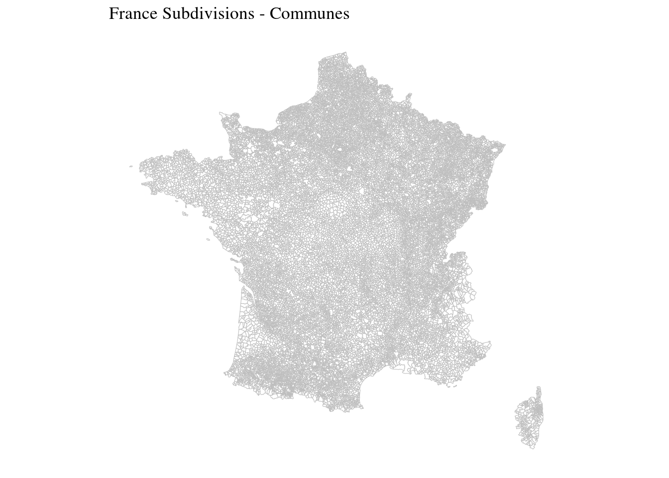

Election choropleth

We have election results per communes and spatial file per communes. It’s time now to merge both datasets and to a choropleth of vote results as % of expressed votes (not counting absent or null votes).

communes_results <- merge(
  x = election_results_sub
  , y = communes_lim_fortified
  , by.x = "code_insee"
  , by.y = "id"
  , allow.cartesian=TRUE
)

A choropleth map (from Greek χῶρος “area/region” and πλῆθος “multitude”) is a thematic map in which areas are shaded or patterned in proportion to the measurement of the statistical variable being displayed on the map, such as population density or per-capita income. (wikipedia)

Finaly we can plot the results with one map per list for the six main lists.

p <- ggplot() +
  geom_polygon(
    data = communes_results, 
    aes(fill = nb_voix_perc_exprimes, x = long, y = lat, group = group),
    color="grey", size = 0.02
  ) +
  scale_fill_viridis_c(option = "A", direction = -1) +
  facet_wrap(facets = . ~ liste_shortname) +
  coord_map() +
  theme_tufte() +
  theme(
    axis.line=element_blank()
    , axis.text=element_blank()
    , axis.ticks=element_blank()
    , axis.title=element_blank()
    ) +
  ggtitle("European election - 2019 - France") +
  labs(fill = "% of votes")
p

References

https://www.r-graph-gallery.com/327-chloropleth-map-from-geojson-with-ggplot2.html