By Datapleth.io | October 11, 2015
In this article we are going to plot a simple map of China with different levels of subdivisions using both base and ggplot2 systems.
In a nutshell, we will have first to get shape files with different subdivision levels, then a bit of data cleaning will be necessary in order to get proper provinces Chinese names. Finally we will plot China base map with subdivisions and add subdivisions names on the map.
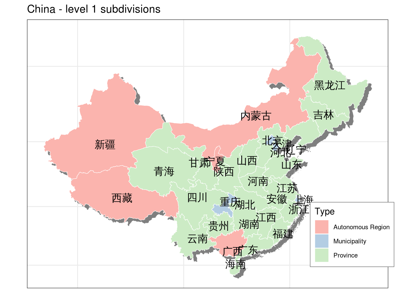
We should obtain the following image as a final result :
Requirements
A lot of geographical models are available online, they need a bit of data processing to be usable in R depending on their format. But first of all we need a set of graphical and data manipulation libraries.
library(maptools)
library(rgeos)
library(gpclib)
library(foreign)
library(sp)
library(ggplot2)
library(plyr)
library(dplyr)
library(RColorBrewer)
About R SpatialPolygonsDataFrame
We need then to get geographical data for China. There are many possible references but we will focus on the commonly used “Global Administrative Areas”, which can be found at http://www.gadm.org/country .
GADM is a spatial database of the location of the world’s administrative areas (or adminstrative boundaries) for use in GIS and similar software. Administrative areas in this database are countries and lower level subdivisions such as provinces, departments…
For instance, if we take China, the first level of subdivisions contains 31 elements of type Province, Municipality, Autonomous Region such as Jiangsu province, Shanghai municipality, etc…
In R, we need to create an object of class SpatialPolygonsDataFrame, this is a
special type of data frame composed of two elements :
- data : basically a data.frame with data associated to available subdivisions (id, name in different languages, type of subdivisions, etc…)
- polygons : a list with as many elements as we have subdivisions (eg. 31 in the case of Chine level 1) with all geographical coordinates for the subdivisions
- more information available here : http://www.inside-r.org/packages/cran/sp/docs/getSpPPolygonsIDSlots
Getting Shapefiles
GADM provides several formats of data, the easiest way is to get directly the data in R format.
A “R SpatialPolygonsDataFrame” (.rds) file can be used in R. To use it, first load the sp package using library(sp) and then use readRDS(“filename.rds”)
But let’s try to work first with shape files as these type of data are widely use by other GIS system and it’s important to learn how to process these.
A “shapefile” consist of at least four actual files (.shp, .shx, .dbf, .prj). This is a commonly used format that can be directly used in Arc-anything, DIVA-GIS, and many other programs.
Let’s download China shapefiles from here : http://biogeo.ucdavis.edu/data/gadm2.7/shp/CHN_adm.zip
We don’t integrate the download scripts and unzip as from China internet access
can be bumpy. We will use then readShapeSpatial method from the maptools
library to load the shapefile of first level subdivisions of China.
# download shapefile
URL <- c("https://data.datapleth.io/ext/GAA/CHN_adm1.shp",
         "https://data.datapleth.io/ext/GAA/CHN_adm1.dbf",
         "https://data.datapleth.io/ext/GAA/CHN_adm1.shx")
destFiles <- c("./data/CHN_adm1.shp",
               "./data/CHN_adm1.dbf",
               "./data/CHN_adm1.shx")

for(i in 1:length(URL)){
    download.file(url = URL[i], destfile = destFiles[i],
                  method = "wget", quiet = FALSE,
                  mode = "w", cacheOK = TRUE)
}
ChinaPolygonsLevel1 <-rgdal::readOGR(dsn =  "./data/CHN_adm1.shp")
## OGR data source with driver: ESRI Shapefile
## Source: "/home/travis/build/longwei66/datapleth/content/blog/data/CHN_adm1.shp", layer: "CHN_adm1"
## with 31 features
## It has 9 fields
## Integer64 fields read as strings: ID_0 ID_1Exploring the data
As mentioned previously, this object has two main parts, the data of subdivisions and the polygons.
str(ChinaPolygonsLevel1@data)## 'data.frame': 31 obs. of 9 variables:
## $ ID_0 : Factor w/ 1 level "49": 1 1 1 1 1 1 1 1 1 1 ...
## $ ISO : Factor w/ 1 level "CHN": 1 1 1 1 1 1 1 1 1 1 ...
## $ NAME_0 : Factor w/ 1 level "China": 1 1 1 1 1 1 1 1 1 1 ...
## $ ID_1 : Factor w/ 31 levels "1","10","11",..: 1 12 23 26 27 28 29 30 31 2 ...
## $ NAME_1 : Factor w/ 31 levels "Anhui","Beijing",..: 1 2 3 4 5 6 7 8 9 10 ...
## $ TYPE_1 : Factor w/ 3 levels "Shěng","Zhíxiáshì",..: 1 2 2 1 1 1 3 1 1 1 ...
## $ ENGTYPE_1: Factor w/ 3 levels "Autonomous Region",..: 3 2 2 3 3 3 1 3 3 3 ...
## $ NL_NAME_1: Factor w/ 31 levels "上海|上海","內蒙古自治區|内蒙古自治区",..: 7 3 27 23 22 11 12 25 19 16 ...
## $ VARNAME_1: Factor w/ 31 levels "Ānhuī","Běijīng",..: 1 2 3 4 5 6 7 8 9 10 ...Basically there are 31 subdivisions. We can get their names in local and English languages.
head(unique(ChinaPolygonsLevel1@data$NAME_1))## [1] Anhui Beijing Chongqing Fujian Gansu Guangdong
## 31 Levels: Anhui Beijing Chongqing Fujian Gansu Guangdong Guangxi ... Zhejianghead(unique(ChinaPolygonsLevel1@data$VARNAME_1))## [1] Ānhuī Běijīng Chóngqìng Fújiàn Gānsù Guǎngdōng
## 31 Levels: Ānhuī Běijīng Chóngqìng Fújiàn Gānsù Guǎngdōng ... Zhèjiānghead(unique(ChinaPolygonsLevel1@data$NL_NAME_1))## [1] 安徽|安徽 北京|北京 重慶|重庆 福建 甘肅|甘肃 廣東|广东
## 31 Levels: 上海|上海 內蒙古自治區|内蒙古自治区 北京|北京 吉林 ... 黑龙江省|黑龍江省Regarding the polygons, we can plot it quickly :
plot(ChinaPolygonsLevel1, main = "China level 1")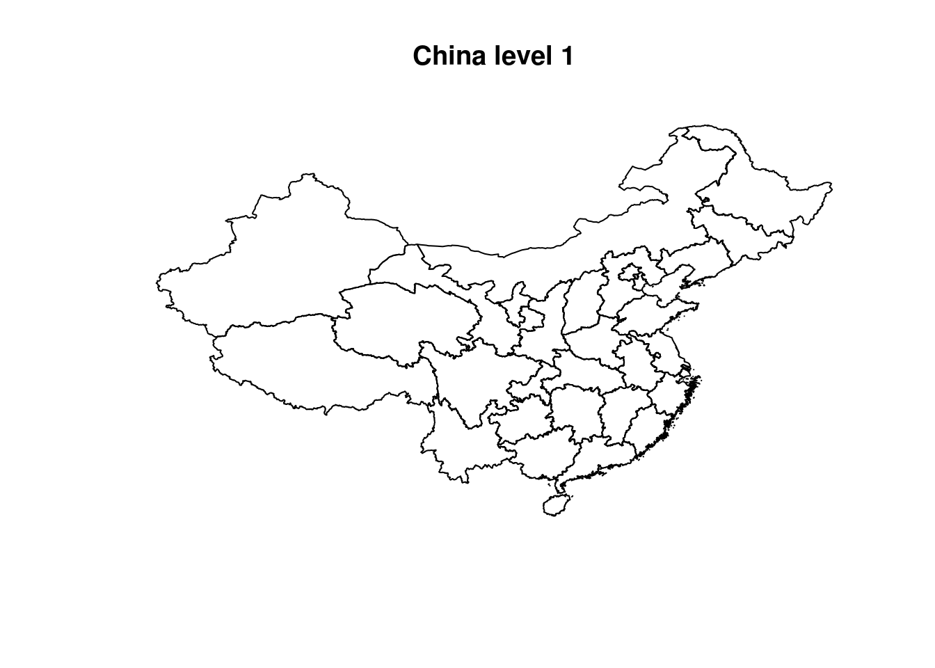
Cleaning data
We would like a clean dataset with proper names in English and Chinese (simplified characters only), thus we need to make few substitutions.
There are some province which names is recorded with both simplified and complex
characters schemes separated by a |
unique(ChinaPolygonsLevel1@data[grep("\\|", ChinaPolygonsLevel1@data$NL_NAME_1),]$NL_NAME_1)## [1] 安徽|安徽 北京|北京
## [3] 重慶|重庆 甘肅|甘肃
## [5] 廣東|广东 廣西壯族自治區|广西壮族自治区
## [7] 貴州|贵州 黑龙江省|黑龍江省
## [9] 江蘇|江苏 遼寧|辽宁
## [11] 內蒙古自治區|内蒙古自治区 寧夏回族自治區|宁夏回族自治区
## [13] 陝西|陕西 山東|山东
## [15] 上海|上海 天津|天津
## [17] 新疆維吾爾自治區|新疆维吾尔自治区 西藏自治區|西藏自治区
## [19] 雲南|云南
## 31 Levels: 上海|上海 內蒙古自治區|内蒙古自治区 北京|北京 吉林 ... 黑龙江省|黑龍江省So let’s substitute these with proper names and simplify also the full names of others.
## Chinese names
ChinaPolygonsLevel1@data$NL_NAME_1 <- gsub("^.*\\|", "", ChinaPolygonsLevel1@data$NL_NAME_1)
ChinaPolygonsLevel1@data[grep("黑龍江省", ChinaPolygonsLevel1@data$NL_NAME_1),]$NL_NAME_1 <- "黑龙江"
ChinaPolygonsLevel1@data[grep("新疆维吾尔自治区", ChinaPolygonsLevel1@data$NL_NAME_1),]$NL_NAME_1 <- "新疆"
ChinaPolygonsLevel1@data[grep("内蒙古自治区", ChinaPolygonsLevel1@data$NL_NAME_1),]$NL_NAME_1 <- "内蒙古"
ChinaPolygonsLevel1@data[grep("宁夏回族自治区", ChinaPolygonsLevel1@data$NL_NAME_1),]$NL_NAME_1 <- "宁夏"
ChinaPolygonsLevel1@data[grep("广西壮族自治区", ChinaPolygonsLevel1@data$NL_NAME_1),]$NL_NAME_1 <- "广西"
ChinaPolygonsLevel1@data[grep("西藏自治区", ChinaPolygonsLevel1@data$NL_NAME_1),]$NL_NAME_1 <- "西藏"

## English names
ChinaPolygonsLevel1@data$NAME_1 <- as.character(ChinaPolygonsLevel1@data$NAME_1)
ChinaPolygonsLevel1@data[grep("Xinjiang Uygur", ChinaPolygonsLevel1@data$NAME_1),]$NAME_1 <- "Xinjiang"
ChinaPolygonsLevel1@data[grep("Nei Mongol", ChinaPolygonsLevel1@data$NAME_1),]$NAME_1 <- "Nei Menggu"
ChinaPolygonsLevel1@data[grep("Ningxia Hui", ChinaPolygonsLevel1@data$NAME_1),]$NAME_1 <- "Ningxia"
ChinaPolygonsLevel1@data$NAME_1 <- as.factor(ChinaPolygonsLevel1@data$NAME_1)
Here is the final list in simplified Chinese : 安徽, 北京, 重庆, 福建, 甘肃, 广东, 广西, 贵州, 海南, 河北, 黑龙江, 河南, 湖北, 湖南, 江苏, 江西, 吉林, 辽宁, 内蒙古, 宁夏, 青海, 陕西, 山东, 上海, 山西, 四川, 天津, 新疆, 西藏, 云南, 浙江
Here is the final list in English : Anhui, Beijing, Chongqing, Fujian, Gansu, Guangdong, Guangxi, Guizhou, Hainan, Hebei, Heilongjiang, Henan, Hubei, Hunan, Jiangsu, Jiangxi, Jilin, Liaoning, Nei Menggu, Ningxia, Qinghai, Shaanxi, Shandong, Shanghai, Shanxi, Sichuan, Tianjin, Xinjiang, Xizang, Yunnan, Zhejiang
Prepare ggplot maps : Converting spacial polygon shapes to data frame
Later we will use ggplot to plot China maps, we need to convert the polygons
object into data frame with fortify function. Region will be identified by
names in simplified Chinese.
# Convert the spacial polygon shapes to data frame
# Use level1 as index
ChinaLevel1Data <- ChinaPolygonsLevel1@data
ChinaLevel1Data$id <- ChinaLevel1Data$NL_NAME_1

# Fortify the data (polygon map as dataframe)
ChinaLevel1dF <- ggplot2::fortify(ChinaPolygonsLevel1, region = "NL_NAME_1")
First map of China with level 1 subdivisions with ggplot
Let’s make our first China ggplot map, we fill subdivisions depending on their types and their borders are colored based on type in Chinese. For this version we use the geom_map() function.
## Now we can make a simple map
g <- ggplot() +
    geom_map(data = ChinaLevel1Data, aes(map_id = id, fill = ENGTYPE_1, col = TYPE_1), map = ChinaLevel1dF) +
    expand_limits(x = ChinaLevel1dF$long, y =  ChinaLevel1dF$lat) +
    coord_map() +
    labs(x="Longitude", y="Latitude", title="Map of China level 1 subdivisions per type (using ggplot)") +
    theme_bw()
print(g)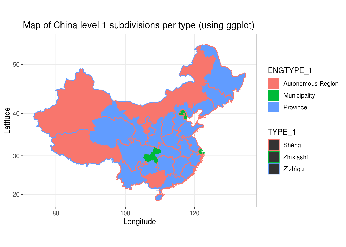
An alternative way is to merge all data in one data set and use a different approach for plotting the polygons (see references).
## Merge polygons and associated data in one data frame by id (name of the province in chinese)
ChinaLevel1 <- merge(ChinaLevel1dF, ChinaLevel1Data, by = "id")

## Create the ggplot using standard approach
## group is necessary to draw in correct order, try without to understand the problem
g <- ggplot(ChinaLevel1, aes(x = long, y = lat, fill = ENGTYPE_1, group = group))
## projected shadow
g <- g+ geom_polygon(aes(x = long + 0.7, y = lat - 0.5), color = "grey50", size = 0.2, fill = "grey50")
## Province boundaries
g <- g + geom_polygon(color = "white", size = 0.2)
## to keep correct ratio in the projection
g <- g + coord_map()
g <- g + labs(title = "China - level 1 subdivisions")
print(g)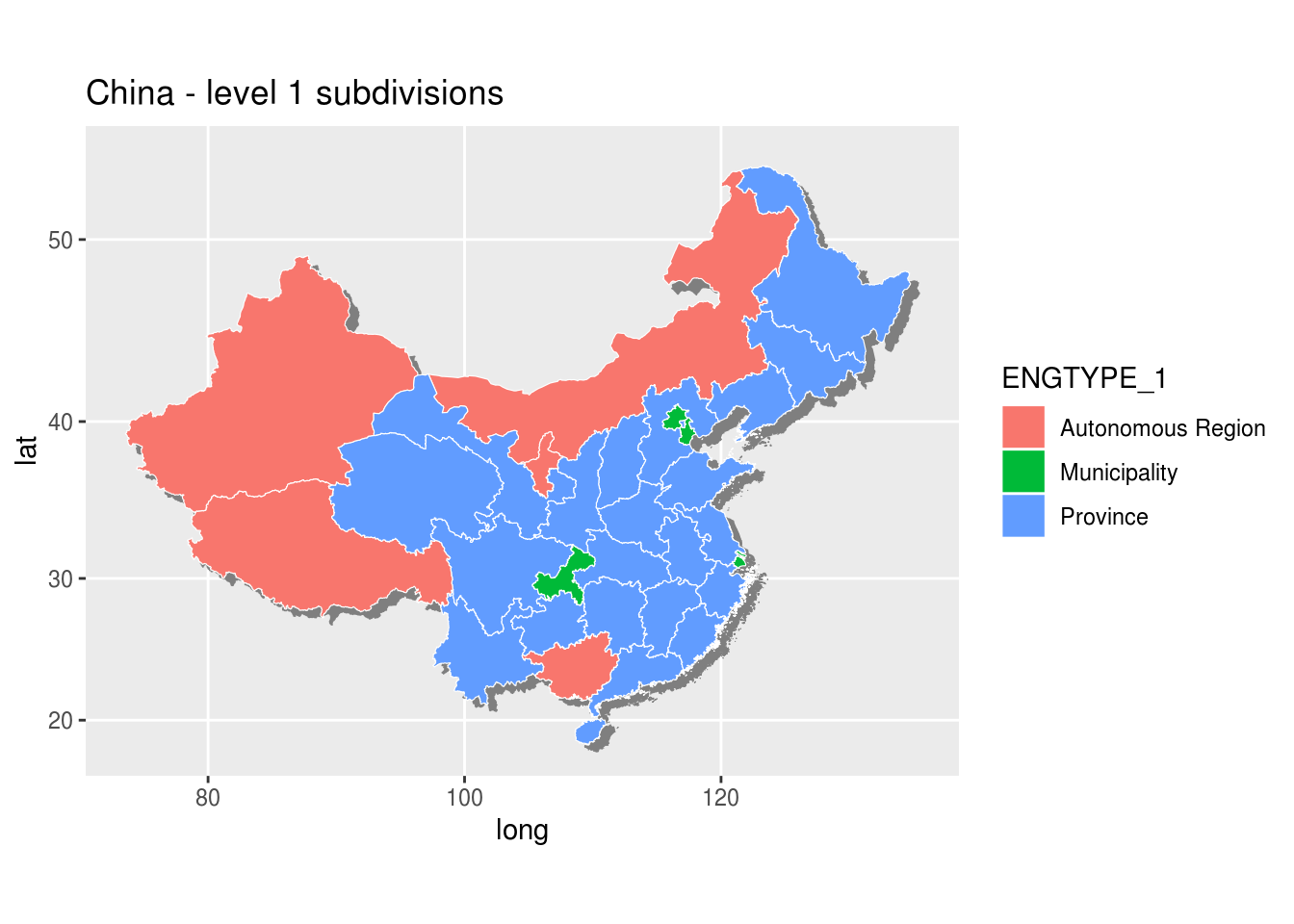
We want to plot province names, for that let’s calculate the theoretical center of each province.
## Getting the center of each subdivision (to plot names or others)
Level1Centers <-
    plyr::ddply(ChinaLevel1dF, .(id), summarize, clat = mean(lat), clong = mean(long))
## Merge results in one data frame
ChinaLevel1Data <- merge(ChinaLevel1Data, Level1Centers, all = TRUE)
Let’s add the names on the previous map, we change the color fill using one of palettes available : http://www.cookbook-r.com/Graphs/Colors_%28ggplot2%29/
## Add the province chinese names
h <- g + geom_text(data = ChinaLevel1Data ,
                   aes(
                       x = jitter(clong, amount = 1),
                       y = jitter(clat, amount = 1),
                       label = id, size = 0.2,
                       group = NULL, fill=NULL
                   ),
                   show.legend = FALSE
)

## Theme configuration
h <- h + theme_bw() +
    theme(axis.text = element_blank(),
          axis.title = element_blank(),
          axis.ticks = element_blank(),
          legend.position = c(0.9, 0.2),
          legend.text = element_text(size = rel(0.7)),
          legend.background = element_rect(color = "gray50", size = 0.3,
                                           fill = "white"))

## Change Palette
h <- h + scale_fill_brewer(palette="Pastel1", name="Type")
print(h)
Code information
There are three excellent reference article (with maps of Nepal and Toronto) for such process :
- http://bl.ocks.org/prabhasp/raw/5030005/
- http://unconj.ca/blog/choropleth-maps-with-r-and-ggplot2.html
- http://rpsychologist.com/working-with-shapefiles-projections-and-world-maps-in-ggplot
In addition the source code of this post is available on github
Our session information :
sessionInfo()## R version 3.6.1 (2017-01-27)
## Platform: x86_64-pc-linux-gnu (64-bit)
## Running under: Ubuntu 16.04.6 LTS
##
## Matrix products: default
## BLAS: /home/travis/R-bin/lib/R/lib/libRblas.so
## LAPACK: /home/travis/R-bin/lib/R/lib/libRlapack.so
##
## locale:
## [1] LC_CTYPE=en_US.UTF-8 LC_NUMERIC=C
## [3] LC_TIME=en_US.UTF-8 LC_COLLATE=en_US.UTF-8
## [5] LC_MONETARY=en_US.UTF-8 LC_MESSAGES=en_US.UTF-8
## [7] LC_PAPER=en_US.UTF-8 LC_NAME=C
## [9] LC_ADDRESS=C LC_TELEPHONE=C
## [11] LC_MEASUREMENT=en_US.UTF-8 LC_IDENTIFICATION=C
##
## attached base packages:
## [1] stats graphics grDevices utils datasets methods base
##
## other attached packages:
## [1] RColorBrewer_1.1-2 dplyr_0.8.3 plyr_1.8.5 ggplot2_3.2.1
## [5] foreign_0.8-72 gpclib_1.5-5 rgeos_0.5-2 maptools_0.9-9
## [9] sp_1.3-2
##
## loaded via a namespace (and not attached):
## [1] Rcpp_1.0.3 compiler_3.6.1 pillar_1.4.2 tools_3.6.1
## [5] digest_0.6.23 evaluate_0.14 lifecycle_0.1.0 tibble_2.1.3
## [9] gtable_0.3.0 lattice_0.20-38 pkgconfig_2.0.3 rlang_0.4.2
## [13] mapproj_1.2.6 rgdal_1.4-8 yaml_2.2.0 blogdown_0.17.1
## [17] xfun_0.11 withr_2.1.2 stringr_1.4.0 knitr_1.26
## [21] maps_3.3.0 grid_3.6.1 tidyselect_0.2.5 glue_1.3.1
## [25] R6_2.4.1 rmarkdown_1.18 bookdown_0.16 farver_2.0.1
## [29] purrr_0.3.3 magrittr_1.5 scales_1.1.0 htmltools_0.4.0
## [33] assertthat_0.2.1 colorspace_1.4-1 labeling_0.3 stringi_1.4.3
## [37] lazyeval_0.2.2 munsell_0.5.0 crayon_1.3.4