About pollution,particle matters, PM2.5, Beijing vs. Shanghai and other cities - Part 1

Definition and reference

What is AQI ? From airnow.gov

The AQI is an index for reporting daily air quality. It tells you how clean or polluted your air is, and what associated health effects might be a concern for you.

EPA (United States Environmental Protection Agency) calculates the AQI for five major air pollutants. The AQI is the highest value calculated for each pollutant as follows: Ozone, PM2.5, PM10, CO, SO2, NO2. In China the main matter is from far the PM2.5 pollutant.

What is the PM2.5 ? From airnow.gov

Particle pollution, also called particulate matter or PM, is a mixture of solids and liquid droplets floating in the air. Some particles are released directly from a specific source, while others form in complicated chemical reactions in the atmosphere. Particles come in a wide range of sizes. Fine particles (PM2.5) are 2.5 micrometers in diameter or smaller, and can only be seen with an electron microscope. Fine particles are produced from all types of combustion, including motor vehicles, power plants, residential wood burning, forest fires, agricultural burning, and some industrial processes. Numerous scientific studies connect particle pollution exposure to a variety of health issues

PM2.5 particles are measured by sensors which provide readings in micro grams per cubic meter of air.

We are going to use the american standard which is the most recognized internationally. We will discuss in the second part the difference with the Chinese standard and its impact on our conclusions. The reference document for AQI reporting is “Technical Assistance Document for the Reporting of Daily Air Quality – the Air Quality Index (AQI)” from the U.S. Environmental Protection Agency EPA-454/B-13-001 of December 2013

AQI index and PM2.5 R functions

To understand AQI levels depending on concentration of particles, we need to understand the function to convert PM2.5 concentration to AQI index. It is linear with several breakpoints defined in US standard. The last breakpoints is matching 500 ppm PM2.5, we will use the same slope as last band for concentration above this point. A comparison with Chinese standard will be shown in the second part of this post.

## Concentration to AQI
pm25_to_aqi <- function(Cp, standard = "US"){
  if(is.na(Cp) | Cp < 0){
    Ip <- NA} else {
      if(standard=="US"){ ## Configure AQI banding, ref  EPA-454/B-13-001, December 2013
        bandsUS <- as.data.frame(rbind(
          c(12,0,50,0),
          c(35.4,12.1,100,51),
          c(55.4,35.5,150,101),
          c(150.4,55.5,200,151),
          c(250.4,150.5,300,201),
          c(350.4,250.5,400,301),
          c(500.4,350.5,500,401)))
        names(bandsUS) <- c("BPhi", "BPlo", "Ih", "Ilo")}
      
      ## Get BPhi, BPlo, Calculate AQI
      if(Cp <= 500.4) {
        BPlo <- max(bandsUS[Cp >= bandsUS$BPlo,]$BPlo)
        Ilo <- max(bandsUS[Cp >= bandsUS$BPlo,]$Ilo)
        BPhi <- min(bandsUS[Cp <= bandsUS$BPhi,]$BPhi)
        Ih <- min(bandsUS[Cp <= bandsUS$BPhi,]$Ih)
        Ip <- (Ih-Ilo)/(BPhi-BPlo)*(Cp-BPlo)+Ilo
      } else {
        Ip <- (500-401)/(500.4-350.5)*(Cp-500.4)+500
      }}
  Ip
} 

Visualisation of relation between AQI and Pm2.5

Using the function defined previously we can illustrate the evolution of AQI level depending on concentration levels of fine particles. We have added the commonly used banding (associated with colors) for AQI.

# generate points from 1 to 500 ppm of PM2.5
a <- (1:1000)/2
curve <- as.data.frame(list("pm2.5" = a, "aqi" = sapply(a,pm25_to_aqi)))
p <- ggplot() + theme_tufte()
st <- 0
alp <- 0.9
p <- p +
  geom_rect(aes(xmin = st, xmax = 500, ymin = 0, ymax = 50), fill = "#00E400",
            alpha = alp) +
  geom_rect(aes(xmin = st, xmax = 500, ymin = 50, ymax = 100), fill = "#FFFF00",
            alpha = alp)  +
  geom_rect(aes(xmin = st, xmax = 500, ymin = 100, ymax = 150), fill = "#FF7E00",
            alpha = alp)  +
  geom_rect(aes(xmin = st, xmax = 500, ymin = 150, ymax = 200), fill = "#FF0000",
            alpha = alp) +
  geom_rect(aes(xmin = st, xmax = 500, ymin = 200, ymax = 300), fill = "#8F3F97",
            alpha = alp) +
  geom_rect(aes(xmin = st, xmax = 500, ymin = 300, ymax = 500), fill = "#7E0023",
            alpha = alp) +
  annotate("text", x = rep(480,6), y = c(25,75,125,175,250,380), 
           label = c("Good",
                     "Moderate",
                     "Unhealthy for Sensitive Groups",
                     "Unhealthy",
                     "Very Unhealthy",
                     "Hazardous"
           ), size =5.5, hjust = 1) +
  geom_point(data = curve, aes(x = pm2.5, y = aqi), col = "blue", size = 1) +
  ggtitle("Evolution of AQI vs. PM2.5") +
  xlab("Particule matter, pm2.5 (in micro gram per m3)") +
  ylab("AQI, air quality index") +
  annotate("text", x = 10, y = 480, label = "(c) datapleth.io", col = "white", hjust = 0) +
  coord_fixed()
p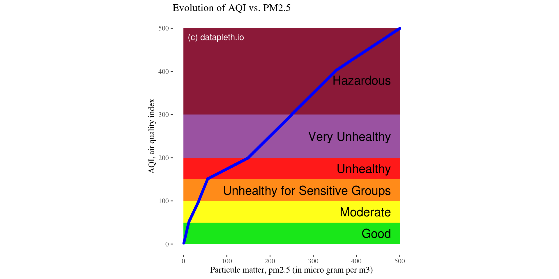 

We can see clearly from the graph above that in the lower concentration of PM2.5 the AQI is increasing fast, 50 micro grams of particles per m3 makes 150 of AQI but then after this point the AQI is increasing slowly. This is important to know in China as AQI is often between 150 and 200, this makes actually a huge gap in term of particle concentration which are respectively between 55 and 150 (three times more!).

Notes about averaging, nowcast and instantcast

Effect on health of particle matters are know and studied for 24h averages. This short article explains the problem.

The concept behind the nowcast is to compensate the “24 hours averaging”, which should be used when converting concentrations to AQI. The reason for this averaging is that the AQI scale specifies that each of the Levels of Health Concern (i.e. Good, Moderate,… Unhealthy…) is valid under a 24 hours exposure[1]. For example, when seeing a 188 AQI (Unhealthy), one need to read it as “if I stay out for 24 hours, and the AQI is 188 during those 24 hours, then the health effect is Unhealthy”. This is quite different from saying that “if the AQI reported now is 188, then the health effect is Unhealthy”.

As the dynamic of air pollution can be very active in China (especially in Beijing), we will not use any averaging in our studies and use the instant readings (instantcast).

Function to download aqi data files

We build a function which download a set of URL and store them in a directory. The download is only done if the file does not exists.

downloadIF <- function(url,file,folder) {
  # generate full file name
  fileName <- paste(folder,file,sep = "/")
  # Download only if file does not exists
  if(!file.exists(fileName)){
    message(url)
    download.file(url = url, destfile = fileName, 
                  method = "wget", quiet = FALSE,
                  mode = "w", cacheOK = TRUE)
    FALSE } else {TRUE} }

Available data for China

From the US website about AQI data in China http://www.stateair.net, we have created a csv file of available url of data sources for the cities of : Beijing, Shanghai, Chengdu, Guangzhou and Shenyang. Please note that not all cities have data available before 2013.

This url list is available in our git repo

# get from github
aqiChinaDatasources <- fread(
  "https://raw.githubusercontent.com/longwei66/dataPleth-wordpress/master/data/share/aqi/aqi-cities-data-source-url.csv", 
  header = TRUE, stringsAsFactors = FALSE)
aqiChinaDatasources$folder <- paste(
  "./data/",
  aqiChinaDatasources$country,
  aqiChinaDatasources$city,sep="/")
aqiChinaDatasources$file <- gsub("(.*)\\/", "", aqiChinaDatasources$url)

Download data for China

check <- NULL
for(i in 1:nrow(aqiChinaDatasources)){
  check <- c(check,
             downloadIF(
               url = aqiChinaDatasources$url[i],
               file = aqiChinaDatasources$file[i],
               folder = "./data/"
               #folder = aqiChinaDatasources$folder[i])
             ))
}

## http://www.stateair.net/web/assets/historical/1/Beijing_2008_HourlyPM2.5_created20140325.csv

## http://www.stateair.net/web/assets/historical/1/Beijing_2009_HourlyPM25_created20140709.csv

## http://www.stateair.net/web/assets/historical/1/Beijing_2010_HourlyPM25_created20140709.csv

## http://www.stateair.net/web/assets/historical/1/Beijing_2011_HourlyPM25_created20140709.csv

## http://www.stateair.net/web/assets/historical/1/Beijing_2012_HourlyPM2.5_created20140325.csv

## http://www.stateair.net/web/assets/historical/1/Beijing_2013_HourlyPM2.5_created20140325.csv

## http://www.stateair.net/web/assets/historical/1/Beijing_2014_HourlyPM25_created20150203.csv

## http://www.stateair.net/web/assets/historical/1/Beijing_2015_HourlyPM25_created20160201.csv

## http://www.stateair.net/web/assets/historical/1/Beijing_2016_HourlyPM25_created20170201.csv

## http://www.stateair.net/web/assets/historical/1/Beijing_2017_HourlyPM25_created20170803.csv

## http://www.stateair.net/web/assets/historical/1/Shanghai_2011_HourlyPM25_created20140423.csv

## http://www.stateair.net/web/assets/historical/1/Shanghai_2012_HourlyPM25_created20140423.csv

## http://www.stateair.net/web/assets/historical/1/Shanghai_2013_HourlyPM25_created20140423.csv

## http://www.stateair.net/web/assets/historical/1/Shanghai_2014_HourlyPM25_created20150203.csv

## http://www.stateair.net/web/assets/historical/1/Shanghai_2015_HourlyPM25_created20160201.csv

## http://www.stateair.net/web/assets/historical/1/Shanghai_2016_HourlyPM25_created20170201.csv

## http://www.stateair.net/web/assets/historical/1/Shanghai_2017_HourlyPM25_created20170803.csv

## http://www.stateair.net/web/assets/historical/1/Chengdu_2012_HourlyPM25_created20140423.csv

## http://www.stateair.net/web/assets/historical/1/Chengdu_2013_HourlyPM25_created20140423.csv

## http://www.stateair.net/web/assets/historical/1/Chengdu_2014_HourlyPM25_created20150203.csv

## http://www.stateair.net/web/assets/historical/1/Chengdu_2015_HourlyPM25_created20160201.csv

## http://www.stateair.net/web/assets/historical/1/Chengdu_2016_HourlyPM25_created20170201.csv

## http://www.stateair.net/web/assets/historical/1/Chengdu_2017_HourlyPM25_created20170803.csv

## http://www.stateair.net/web/assets/historical/1/Guangzhou_2011_HourlyPM25_created20140423.csv

## http://www.stateair.net/web/assets/historical/1/Guangzhou_2012_HourlyPM25_created20140423.csv

## http://www.stateair.net/web/assets/historical/1/Guangzhou_2013_HourlyPM25_created20140423.csv

## http://www.stateair.net/web/assets/historical/1/Guangzhou_2014_HourlyPM25_created20150203.csv

## http://www.stateair.net/web/assets/historical/1/Guangzhou_2015_HourlyPM25_created20160201.csv

## http://www.stateair.net/web/assets/historical/1/Guangzhou_2016_HourlyPM25_created20170201.csv

## http://www.stateair.net/web/assets/historical/1/Guangzhou_2017_HourlyPM25_created20170803.csv

## http://www.stateair.net/web/assets/historical/1/Shenyang_2013_HourlyPM25_created20140423.csv

## http://www.stateair.net/web/assets/historical/1/Shenyang_2014_HourlyPM25_created20150203.csv

## http://www.stateair.net/web/assets/historical/1/Shenyang_2015_HourlyPM25_created20160201.csv

## http://www.stateair.net/web/assets/historical/1/Shenyang_2016_HourlyPM25_created20170201.csv

## http://www.stateair.net/web/assets/historical/1/Shenyang_2017_HourlyPM25_created20170803.csv

On a total of 35 url, we downloaded 35 file(s) and 0 files were already in our folder.

China

# Function to read AQI data from csv file to data.frame
load_aqi_data <- function(filepath,mycountry,mycity,myyear) {
  dF <-fread(
    filepath, sep = ",", header = FALSE, stringsAsFactors = FALSE, 
    strip.white = TRUE, skip = 3)
  ## return the dataframe of AQI data, fix variable names
  setnames(dF, make.names(dF[1]))
  dF <- dF[2:nrow(dF)]
  dF[ , ':=' (
    country = mycountry,
    city = mycity,
    year = myyear
    ) ]
  dF
  }
# Function to read a bunch of csv files specified in a vector and return on list of data.frames
aqi <- NULL
for(i in 1:nrow(aqiChinaDatasources)){
  # extract file name (end of url)
  filepath <- paste("./data/",
                    aqiChinaDatasources$file[i],sep = "/")
  message(filepath)
  aqi <- rbind(aqi,
               load_aqi_data(filepath = filepath,
                             mycountry = aqiChinaDatasources$country[i],
                             mycity = aqiChinaDatasources$city[i],
                             myyear = aqiChinaDatasources$year[i]))
  message(nrow(aqi))
}

# Site
# is equivalent to city, we won't keep it
sum(aqi$Site == aqi$city) - nrow(aqi)

## [1] 0

# Parameter
# There are only PM2.5 readings in the data set, we won't keep the column
unique(aqi$Parameter)

## [1] "PM2.5"

# Date..LST.
# the format of 2015 and other year is different
# some are in YYYY-MM-DD
format1 <-  sum(grepl(pattern = "^20[0-9][0-9]-.*",x = aqi$Date..LST.))
# some are in D/M/YYYY
format2 <- sum(grepl(pattern = ".*\\/.*\\/20[0-9][0-9]",x = aqi$Date..LST.))
# These two formats covers the dataset
format1 + format2 - nrow(aqi)

## [1] 0

# we convert the character string as "POSIXlt" "POSIXt"
# for each form
aqi$date.time <- as.POSIXct(strptime("2000-12-31 12:00", "%Y-%m-%d %H:%M"))
testFormat1 <- grepl(pattern = "^20[0-9][0-9]-.*",x = aqi$Date..LST.)
testFormat2 <- grepl(pattern = ".*\\/.*\\/20[0-9][0-9]",x = aqi$Date..LST.)
aqi[testFormat1]$date.time <- as.POSIXct(strptime(aqi[testFormat1,]$Date..LST., "%Y-%m-%d %H:%M"))
aqi[testFormat2]$date.time <- as.POSIXct(strptime(aqi[testFormat2,]$Date..LST., "%m/%d/%Y %H:%M"))
summary(aqi$date.time)

##                  Min.               1st Qu.                Median 
## "2008-04-08 15:00:00" "2012-08-10 16:00:00" "2014-04-16 21:00:00" 
##                  Mean               3rd Qu.                  Max. 
## "2014-02-08 16:44:36" "2015-11-23 10:00:00" "2017-06-30 23:00:00"

# Nothing to do for year
class(aqi$year)

## [1] "integer"

unique(aqi$year)

##  [1] 2008 2009 2010 2011 2012 2013 2014 2015 2016 2017

# We need to convert month,day in integer
class(aqi$Month); unique(aqi$Month); aqi$Month <- as.numeric(aqi$Month)

## [1] "character"

##  [1] "4"  "5"  "6"  "7"  "8"  "9"  "10" "11" "1"  "2"  "3"  "12"

class(aqi$Day); unique(aqi$Day); aqi$Day <- as.numeric(aqi$Day)

## [1] "character"

##  [1] "8"  "9"  "10" "11" "12" "13" "14" "15" "16" "17" "18" "19" "20" "21" "22"
## [16] "23" "24" "25" "26" "27" "28" "29" "30" "1"  "2"  "3"  "4"  "5"  "6"  "7" 
## [31] "31"

class(aqi$Hour); unique(aqi$Hour); aqi$Hour <- as.numeric(aqi$Hour)

## [1] "character"

##  [1] "15" "16" "17" "18" "19" "20" "21" "22" "23" "0"  "1"  "2"  "3"  "4"  "5" 
## [16] "6"  "7"  "8"  "9"  "10" "11" "12" "13" "14"

# We need to convert Value in integer under the variable pm2.5
aqi$pm2.5 <- as.numeric(aqi$Value)
# Some of the data are not valid as stated in QC.name, these are 0 and -999
# we should replace these by NA
unique(aqi[aqi$QC.Name == "Missing",]$pm2.5)

## [1] -999    0

aqi[aqi$QC.Name == "Missing",]$pm2.5 <- NA
# we notice that some Values are still negatives or -999
# we replace them by NA and update QC.name by missing
aqi[!is.na(aqi$pm2.5) & aqi$pm2.5 < 0,]$QC.Name <- NA
aqi[!is.na(aqi$pm2.5) & aqi$pm2.5 < 0,]$pm2.5 <- NA
# we won't need the parameter Duration
unique(aqi$Duration)

## [1] "1 Hr"

# we won't need the parameter Year as we have year
sum(as.numeric(aqi$Year) == aqi$year) - nrow(aqi)

## [1] 0

# Let's keep only what we need
aqi <- select(aqi,-Site,-Parameter,-Year,-Unit, -Date..LST., -Value, -Duration)
# Let's calculate the aqi index value with the function defined before
aqi$aqi <- sapply(aqi$pm2.5,pm25_to_aqi)
# add one variable for date
aqi$date <- as.character(strptime(paste(aqi$year,aqi$Month,aqi$Day,sep = "-"), "%Y-%m-%d"))
# Let's rename variable and reorder
setnames(aqi, c("month","day","hour","measurement.available","country","city","year","date.time","pm2.5", "aqi","date"))
aqi <- select(aqi, country, city, date.time, date, year, month, day, hour, measurement.available, pm2.5, aqi)

Paris

# Paris
ParisAqi <- fread(parisAQIdatafile, sep = ";", na.strings = "n/d", stringsAsFactors = FALSE, header = FALSE, skip = 2)
setnames(ParisAqi, c("date","heure","PM25","PM10","O3","NO2","CO"))

## create measurement.available column
ParisAqi[ , measurement.available := "Valid"]
ParisAqi[is.na(ParisAqi$PM25), measurement.available := "Missing"]
## create date.time variable
ParisAqi[ , date.time := paste(date, heure, sep = "-")]
## select only the variable we need
ParisAqi <- ParisAqi[, .(date.time, PM25, measurement.available)]
## change names
setnames(ParisAqi, c("date.time", "pm2.5", "measurement.available"))
## convert the character variable to date format
ParisAqi[ , date.time := as.POSIXct(strptime(ParisAqi$date.time, "%d/%m/%Y-%H")) ]

## Warning in strptime(ParisAqi$date.time, "%d/%m/%Y-%H"): strptime() usage
## detected and wrapped with as.POSIXct(). This is to minimize the chance of
## assigning POSIXlt columns, which use 40+ bytes to store one date (versus 8 for
## POSIXct). Use as.POSIXct() (which will call strptime() as needed internally) to
## avoid this warning.

## add reference fields
ParisAqi[ , ':=' (
  country = "France",
  city = "Paris",
  year = as.numeric(year(date.time)),
  month = as.numeric(month(date.time)),
  day = as.numeric(day(date.time)),
  hour = as.numeric(hour(date.time)),
  pm2.5 = as.numeric(pm2.5)
  )]
ParisAqi$aqi <- as.numeric(sapply(ParisAqi$pm2.5,pm25_to_aqi))
# add one variable for date
ParisAqi$date <- as.character(strptime(paste(ParisAqi$year,ParisAqi$month,ParisAqi$day,sep = "-"), "%Y-%m-%d"))
## order the fields
ParisAqi <- ParisAqi[ , .(
  country,city,
  date.time,
  date,
  year,
  month,
  day,
  hour,
  measurement.available,
  pm2.5,
  aqi
  )]